43 add data labels to chart excel
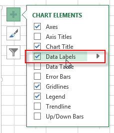
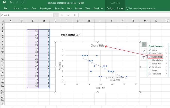
Add data labels excel To add or move data labels in a chart, you can do as below steps: In Excel 2013 or 2016. 1. Click the chart to show the Chart Elements button .. 2. Then click the Chart Elements, and check Data Labels, then you can click the arrow to choose an option about the data labels Add data labels and callouts to charts in Excel 365 | EasyTweaks.com The steps that I will share in this guide apply to Excel 2021 / 2019 / 2016. Step #1: After generating the chart in Excel, right-click anywhere within the chart and select Add labels . Note that you can also select the very handy option of Adding data Callouts.
Add / Move Data Labels in Charts - Excel & Google Sheets Adding Data Labels Click on the graph Select + Sign in the top right of the graph Check Data Labels Change Position of Data Labels Click on the arrow next to Data Labels to change the position of where the labels are in relation to the bar chart Final Graph with Data Labels

Add data labels to chart excel
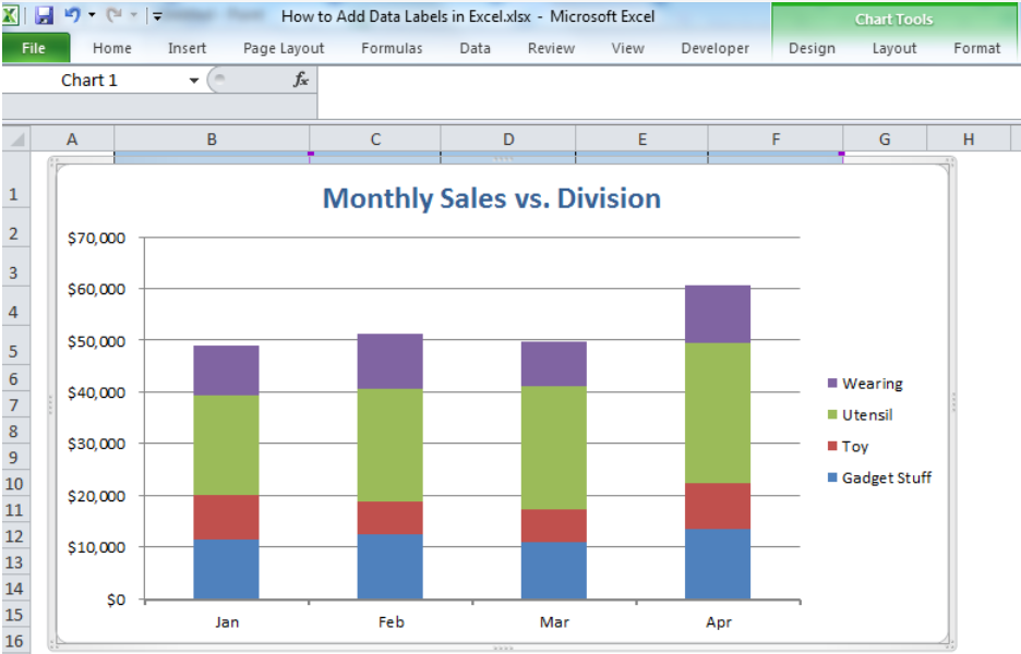
Add a data series to your chart - support.microsoft.com Right-click the chart, and then choose Select Data. The Select Data Source dialog box appears on the worksheet that contains the source data for the chart. Leaving the dialog box open, click in the worksheet, and then click and drag to select all the data you want to use for the chart, including the new data series. How to add total labels to stacked column chart in Excel? Select and right click the new line chart and choose Add Data Labels > Add Data Labels from the right-clicking menu. See screenshot: And now each label has been added to corresponding data point of the Total data series. And the data labels stay at upper-right corners of each column. 5. How to Add Data Labels to an Excel 2010 Chart - dummies Select where you want the data label to be placed. Data labels added to a chart with a placement of Outside End. On the Chart Tools Layout tab, click Data Labels→More Data Label Options. The Format Data Labels dialog box appears.
Add data labels to chart excel. Add or remove data labels in a chart - support.microsoft.com Add data labels to a chart Click the data series or chart. To label one data point, after clicking the series, click that data point. In the upper right corner, next to the chart, click Add Chart Element > Data Labels. To change the location, click the arrow, and choose an option. Adding Data Labels to Your Chart (Microsoft Excel) Select the position that best fits where you want your labels to appear. To add data labels in Excel 2013 or Excel 2016, follow these steps: Activate the chart by clicking on it, if necessary. Make sure the Design tab of the ribbon is displayed. (This will appear when the chart is selected.) Click the Add Chart Element drop-down list. How to add data labels from different column in an Excel chart? Right click the data series in the chart, and select Add Data Labels > Add Data Labels from the context menu to add data labels. 2. Click any data label to select all data labels, and then click the specified data label to select it only in the chart. 3. How to add or move data labels in Excel chart? - ExtendOffice To add or move data labels in a chart, you can do as below steps: In Excel 2013 or 2016. 1. Click the chart to show the Chart Elements button . 2. Then click the Chart Elements, and check Data Labels, then you can click the arrow to choose an option about the data labels in the sub menu. See screenshot:
Change the format of data labels in a chart To get there, after adding your data labels, select the data label to format, and then click Chart Elements > Data Labels > More Options. To go to the appropriate area, click one of the four icons ( Fill & Line, Effects, Size & Properties ( Layout & Properties in Outlook or Word), or Label Options) shown here. Adding Data Labels to Your Chart (Microsoft Excel) For instance, if you are formatting a pie chart, the data can be more difficult to understand if you don't include data labels. To add data labels, follow these steps: Activate the chart by clicking on it, if necessary. Choose Chart Options from the Chart menu. Excel displays the Chart Options dialog box. Make sure the Data Labels tab is selected. how to add data labels into Excel graphs - storytelling with data There are a few different techniques we could use to create labels that look like this. Option 1: The "brute force" technique. The data labels for the two lines are not, technically, "data labels" at all. A text box was added to this graph, and then the numbers and category labels were simply typed in manually. How to Add Labels to Scatterplot Points in Excel - Statology Step 3: Add Labels to Points. Next, click anywhere on the chart until a green plus (+) sign appears in the top right corner. Then click Data Labels, then click More Options…. In the Format Data Labels window that appears on the right of the screen, uncheck the box next to Y Value and check the box next to Value From Cells.
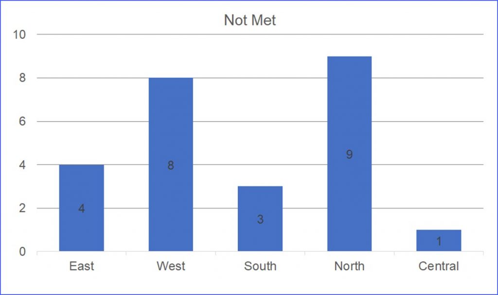
Use a screen reader to add a title, data labels, and a legend to a ... Select the chart that you want to work with. To open the Add Chart Element menu, press Alt+J, C, A. To add data callout labels to the chart, press D and then U. Tip: To remove data labels, select the chart, and then press Alt+J, C, A, D, and then N. Add a legend to a chart Legends help you to quickly understand data relationships in a chart. Adding Data Labels To An Excel Chart - MyExcelOnline In our example below, I add a Data Label to a column chart and then I format the data label using CTRL+1. I then select to custom format the numbers so it shows the values as thousands by adding a comma , after each zero and then showing the work k by adding "k" Example Custom Number Format: [$$-1004]#,##0 ,"k" ;- [$$-1004]#,##0 ,"k" Adding rich data labels to charts in Excel 2013 | Microsoft 365 Blog To add a data label in a shape, select the data point of interest, then right-click it to pull up the context menu. Click Add Data Label, then click Add Data Callout . The result is that your data label will appear in a graphical callout. In this case, the category Thr for the particular data label is automatically added to the callout too. How to Add Data Labels in Excel - Excelchat | Excelchat After inserting a chart in Excel 2010 and earlier versions we need to do the followings to add data labels to the chart; Click inside the chart area to display the Chart Tools. Figure 2. Chart Tools Click on Layout tab of the Chart Tools. In Labels group, click on Data Labels and select the position to add labels to the chart. Figure 3.
Charting in Excel - Adding Data Labels - YouTube
Add a DATA LABEL to ONE POINT on a chart in Excel Click on the chart line to add the data point to. All the data points will be highlighted. Click again on the single point that you want to add a data label to. Right-click and select ' Add data label ' This is the key step! Right-click again on the data point itself (not the label) and select ' Format data label '.

How to Make Excel Charts More Intuitive by Adding Data Labels and Tables - Data Recovery Blog
How to Make a Pie Chart in Excel & Add Rich Data Labels to The Chart! Creating and formatting the Pie Chart. 1) Select the data. 2) Go to Insert> Charts> click on the drop-down arrow next to Pie Chart and under 2-D Pie, select the Pie Chart, shown below. 3) Chang the chart title to Breakdown of Errors Made During the Match, by clicking on it and typing the new title.

How-to Use Data Labels from a Range in an Excel Chart - Excel Dashboard Templates
How to Use Cell Values for Excel Chart Labels Select the chart, choose the "Chart Elements" option, click the "Data Labels" arrow, and then "More Options." Uncheck the "Value" box and check the "Value From Cells" box. Select cells C2:C6 to use for the data label range and then click the "OK" button. The values from these cells are now used for the chart data labels.

Excel: How to make an Excel-lent bull's-eye chart
Apply Custom Data Labels to Charted Points - Peltier Tech First, add labels to your series, then press Ctrl+1 (numeral one) to open the Format Data Labels task pane. I've shown the task pane below floating next to the chart, but it's usually docked off to the right edge of the Excel window. Click on the new checkbox for Values From Cells, and a small dialog pops up that allows you to select a ...

How to Create Multi-Category Chart in Excel - Excel Board
Edit titles or data labels in a chart - support.microsoft.com On a chart, click one time or two times on the data label that you want to link to a corresponding worksheet cell. The first click selects the data labels for the whole data series, and the second click selects the individual data label. Right-click the data label, and then click Format Data Label or Format Data Labels.

Adding Data Labels to Your Chart (Microsoft Excel)
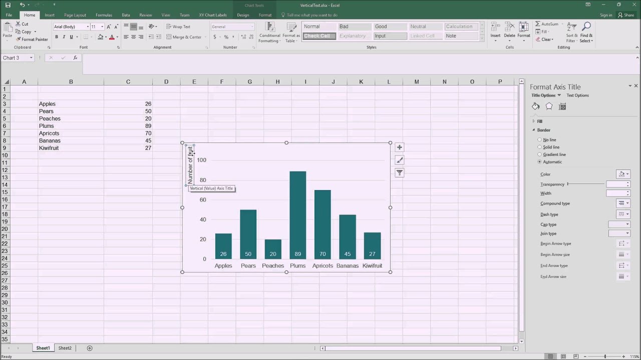
How to add axis label to chart in Excel? - ExtendOffice Select the chart that you want to add axis label. 2. Navigate to Chart Tools Layout tab, and then click Axis Titles, see screenshot: 3.
How to Add Data Labels in Excel - Excelchat | Excelchat
Excel charts: add title, customize chart axis, legend and data labels Click anywhere within your Excel chart, then click the Chart Elements button and check the Axis Titles box. If you want to display the title only for one axis, either horizontal or vertical, click the arrow next to Axis Titles and clear one of the boxes: Click the axis title box on the chart, and type the text.
Adding horizontally-aligned y-axis titles to charts in Excel 2016 - YouTube
Add data labels to your Excel bubble charts | TechRepublic Right-click the data series and select Add Data Labels. Right-click one of the labels and select Format Data Labels. Select Y Value and Center. Move any labels that overlap. Select the data labels...
Excel Charts - Free Excel Tutorial
Custom Chart Data Labels In Excel With Formulas Follow the steps below to create the custom data labels. Select the chart label you want to change. In the formula-bar hit = (equals), select the cell reference containing your chart label's data. In this case, the first label is in cell E2. Finally, repeat for all your chart laebls.
Chart's Data Series in Excel - Easy Excel Tutorial
How to Add Data Labels to an Excel 2010 Chart - dummies Select where you want the data label to be placed. Data labels added to a chart with a placement of Outside End. On the Chart Tools Layout tab, click Data Labels→More Data Label Options. The Format Data Labels dialog box appears.

How to Add Data Labels in Excel - Excelchat | Excelchat
How to add total labels to stacked column chart in Excel? Select and right click the new line chart and choose Add Data Labels > Add Data Labels from the right-clicking menu. See screenshot: And now each label has been added to corresponding data point of the Total data series. And the data labels stay at upper-right corners of each column. 5.
How to Create a Scatter Plot in Excel - TurboFuture - Technology
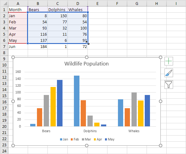
Add a data series to your chart - support.microsoft.com Right-click the chart, and then choose Select Data. The Select Data Source dialog box appears on the worksheet that contains the source data for the chart. Leaving the dialog box open, click in the worksheet, and then click and drag to select all the data you want to use for the chart, including the new data series.
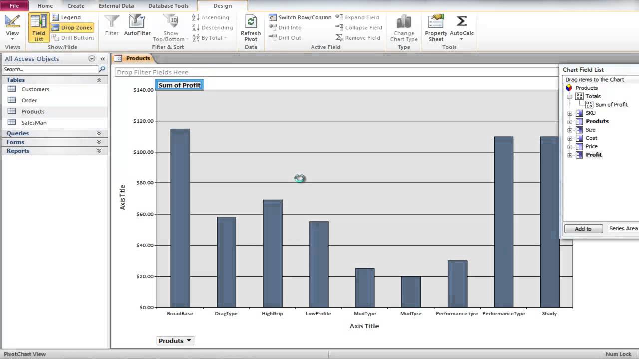
How to Create a Pivot Chart in Microsoft Access - YouTube

How to insert data labels to a Pie chart in Excel 2013 - YouTube
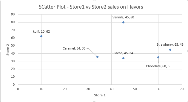
Add Custom Labels to x-y Scatter plot in Excel - DataScience Made Simple
How to Add Data Labels to a Chart - ExcelNotes

Excel Custom Chart Labels • My Online Training Hub
Post a Comment for "43 add data labels to chart excel"